This chapter is a template. It shows prose, maths, numbered theorems, sidenotes, callouts and executed code in one place. Delete it once you have real notes.
1 Setup
Let X_1, X_2, \dots be independent and identically distributed with mean \mu and finite variance \sigma^2. Write the sample mean as
The law of large numbers says \bar{X}_n \to \mu. The central limit theorem describes the fluctuations around that limit.1
Definition 1 (Convergence in distribution) A sequence Y_n converges in distribution to Y, written Y_n \xrightarrow{d} Y, if F_{Y_n}(y) \to F_Y(y) at every point y where F_Y is continuous.
Theorem 1 (Central limit theorem) With \bar{X}_n as in Equation 1,
Proof. Sketch. Standardise so that \mu = 0 and \sigma = 1, and let \varphi be the characteristic function of X_1. Then \varphi(t) = 1 - t^2/2 + o(t^2), so
which is the characteristic function of \mathcal{N}(0,1). Lévy’s continuity theorem finishes the argument.2
NoteWhat the theorem does not say
Theorem 1 needs finite variance. For heavy-tailed distributions such as the Cauchy, the sample mean does not settle down at all.
2 Seeing it numerically
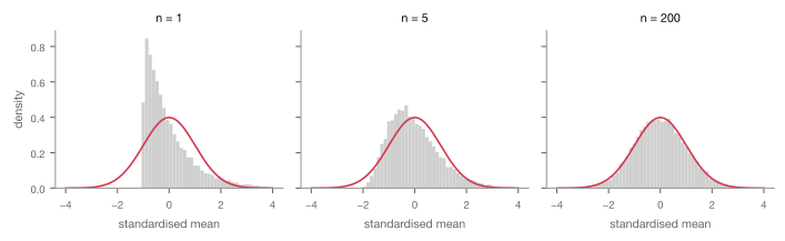
The cell below draws sample means from an exponential distribution, which is strongly skewed, and standardises them as in Theorem 1.
import numpy as nprng = np.random.default_rng(0)def standardised_means(n, reps=20_000):"""Standardised sample means of n Exponential(1) draws, for which mu = sigma = 1.""" x = rng.exponential(scale=1.0, size=(reps, n))return np.sqrt(n) * (x.mean(axis=1) -1.0)for n in (1, 5, 30, 200): z = standardised_means(n) skew = ((z - z.mean()) **3).mean() / z.std() **3print(f"n = {n:>3} mean = {z.mean():+.3f} sd = {z.std():.3f} skew = {skew:+.3f}")
n =   1  mean = -0.007  sd = 0.994  skew = +2.007
n =   5  mean = -0.006  sd = 1.005  skew = +0.906
n =  30  mean = +0.002  sd = 1.005  skew = +0.374
n = 200  mean = -0.010  sd = 1.006  skew = +0.139
The skewness shrinks towards zero as n grows, at the rate in Table 1. Figure 1 shows the same thing.
Quantity
Exact value
Rate
Mean of Z_n
0
none
Variance of Z_n
1
none
Skewness of Z_n
2/\sqrt{n}
n^{-1/2}
Table 1: Moments of the standardised mean Z_n of Exponential(1) draws.
Figure 1: Standardised sample means of Exponential(1) draws against the standard normal density.
3 Exercises
Repeat the experiment with a Bernoulli(0.01) distribution. How large must n be before the histogram looks normal?
Replace the exponential with a standard Cauchy. What happens, and which hypothesis of Theorem 1 fails?
Footnotes
Footnotes are printed in the margin on a wide screen, level with where they are referenced. On a narrow screen, hover or tap the number to read the note in a card.↩︎
A long note is cut off after nine lines with a fade, and shown in full while you hover it or its number. This one is padded to show that: the characteristic function always exists, unlike the moment generating function, which is why the proof is usually written with it. The price is a detour through complex numbers. A proof by moment generating functions is shorter to state but needs every moment to be finite, which rules out many distributions the theorem actually covers. Lindeberg’s replacement argument avoids transforms altogether.↩︎